Linear Regression from Scratch

이 튜토리얼에서는 scikit-learn으로 간단한 선형 회귀 모델을 만들고, 결과를 시각화하고, 모델이 무엇을 학습했는지 이해해 봅니다. 이 노트북은 블로그 포스트 역할도 겸해요 — 여기에 보이는 모든 것, 플롯을 포함해서, 노트북 자체에서 생성된 것입니다.

데이터 생성하기

선형 관계에 약간의 노이즈를 더한 합성 데이터셋을 만들어, 모델의 적합 결과를 실제 정답(ground truth)과 비교할 수 있게 합니다.

import numpy as np
import matplotlib.pyplot as plt
from sklearn.linear_model import LinearRegression
from sklearn.model_selection import train_test_split

rng = np.random.RandomState(42)
X = 2 * rng.rand(100, 1)
y = 4 + 3 * X.ravel() + rng.randn(100) * 0.8

X_train, X_test, y_train, y_test = train_test_split(X, y, test_size=0.2, random_state=42)
print(f'Train samples: {len(X_train)}, Test samples: {len(X_test)}')

Train samples: 80, Test samples: 20

모델 학습하기

이제 ordinary least squares 회귀를 학습하고, 학습된 파라미터를 확인합니다.

model = LinearRegression()
model.fit(X_train, y_train)

print(f'Intercept: {model.intercept_:.3f}')
print(f'Slope: {model.coef_[0]:.3f}')
print(f'R² score on test set: {model.score(X_test, y_test):.3f}')

Intercept: 4.114
Slope: 2.839
R² score on test set: 0.874

적합 결과 시각화하기

아래 플롯은 학습 데이터, 회귀선, 그리고 데이터를 생성할 때 사용한 실제 정답 선을 보여줍니다. 노이즈가 있음에도 적합이 얼마나 가까운지 확인해 보세요.

fig, ax = plt.subplots(figsize=(8, 5))
ax.scatter(X_train, y_train, alpha=0.6, label='Training data')
x_line = np.linspace(0, 2, 100).reshape(-1, 1)
ax.plot(x_line, model.predict(x_line), color='crimson', linewidth=2, label='Regression fit')
ax.plot(x_line, 4 + 3 * x_line.ravel(), color='gray', linestyle='--', linewidth=1.5, label='Ground truth')
ax.set_xlabel('x')
ax.set_ylabel('y')
ax.legend()
ax.set_title('Linear Regression Fit')
plt.tight_layout()
plt.show()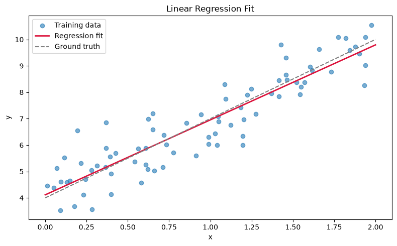

잔차 분석

잔차의 히스토그램은 오차가 대략 정규분포를 따른다는 것을 확인하는 데 도움이 됩니다 — 선형 회귀의 핵심 가정 중 하나예요.

residuals = y_test - model.predict(X_test)

fig, ax = plt.subplots(figsize=(8, 4))
ax.hist(residuals, bins=15, color='steelblue', edgecolor='white')
ax.axvline(0, color='crimson', linestyle='--')
ax.set_xlabel('Residual')
ax.set_ylabel('Count')
ax.set_title('Distribution of Residuals')
plt.tight_layout()
plt.show()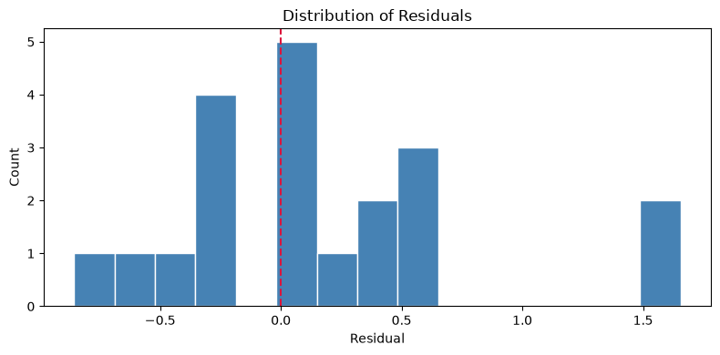

핵심 정리

• 학습된 파라미터(절편 ≈ 4, 기울기 ≈ 3)가 데이터에 심어 둔 실제 관계를 꽤 정확히 복원했습니다.
• 테스트 세트에서 R²가 약 0.9라는 것은 모델이 대부분의 분산을 포착했다는 뜻이에요.
• 잔차가 대략 정규분포를 보이므로, 여기서는 모델 가정이 성립합니다.

다음에는 이를 다중 회귀로 확장하고, 직접 구현한 경사 하강법과 비교해 볼 예정입니다.